Backtesting.py - A complete guide

Backtesting.py is a lightweight backtesting framework in python. It very much takes its syntax from Backtrader. So if you're familiar with Backtrader at all you'll find Backtesting.py very natural and easy to pickup.
Why use Backtesting.py?
Backtesting.py is great when you just want something that works. It's easy to install, has excellent documentation, and doesn't suffer from the bloat of other backtesting libraries with 10,000 different live-trading integrations.
As I mentioned, the syntax will be very familiar to those of you who have used Backtrader. I see it as a spiritual successor to Backtrader, and much more lightweight. It is event-driven, so you program the logic that is run on each bar successively much like you were actually trading the strategy day-to-day.
You can also bring your own indicator libraries, as it doesn't come pre-loaded with any. So feel free to use something lightening fast like TA-lib or something friendly like pandas-ta.
You don't need any data to follow along with this tutorial, as backtesting.py comes pre-loaded with some GOOG daily data that we can use.
The simplest backtest
Here's the code for the simplest possible backtest you can do in backtesting.py.
 1import datetime
 2import pandas_ta as ta
 3import pandas as pd
 4
 5from backtesting import Backtest
 6from backtesting import Strategy
 7from backtesting.lib import crossover
 8from backtesting.test import GOOG
 9
10class RsiOscillator(Strategy):
11
12    upper_bound = 70
13    lower_bound = 30
14    rsi_window = 14
15
16    # Do as much initial computation as possible
17    def init(self):
18        self.rsi = self.I(ta.rsi, pd.Series(self.data.Close), self.rsi_window)
19
20    # Step through bars one by one
21    # Note that multiple buys are a thing here
22    def next(self):
23        if crossover(self.rsi, self.upper_bound):
24            self.position.close()
25        elif crossover(self.lower_bound, self.rsi):
26            self.buy()
27
28bt = Backtest(GOOG, RsiOscillator, cash=10_000, commission=.002)
29stats = bt.run()
30bt.plot()
Make sure you pip install the relevant libraries. I'm using pandas-ta here because it's a little easier to install than ta-lib but the principle is the same.
To get anywhere in Backtesting.py, you need to create a Strategy. You do that by creating a class that inherits from backtesting.Strategy.
There are two main functions you need to worry about inside your strategy. The first is init:
1...
2  # Do as much initial computation as possible
3    def init(self):
4        self.rsi = self.I(ta.rsi, pd.Series(self.data.Close), self.rsi_window)
This function is called as soon as the object is created and is only run once. You should put in here anything that can be pre-calculated ahead of time before your backtest, such as any technical indicators.
The I function is well worth a look at as it's what allows you to build indicators within the backtesting.py ecosystem. Then there's the next function:
1def next(self):
2        if crossover(self.rsi, self.upper_bound):
3            self.position.close()
4        elif crossover(self.lower_bound, self.rsi):
5            self.buy()
next is called on every candle as the backtest progresses. Essentially ask yourself, if you were there at the time of the candle, what would your logic look like. In our case we check if the rsi is above our upper_bound. If it is close any positions we have (long or short). Otherwise check if it's below lower_bound, in which case we should buy as much as we can of the asset. Note that backtesting.py only buys whole numbers of shares.
Finally we run the backtest:
1bt = Backtest(GOOG, RsiOscillator, cash=10_000, commission=.002)
2stats = bt.run()
3bt.plot()
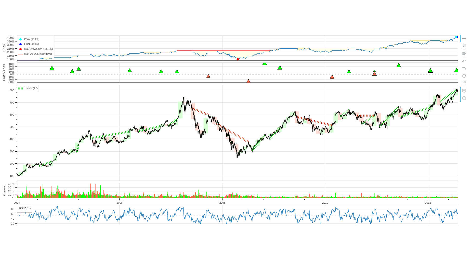
Which should open up a nice backtesting dashboard in your browser.

You can also print out stats to get a nice overview of your strategy and common metrics:
 1Start                     2004-08-19 00:00:00
 2End                       2013-03-01 00:00:00
 3Duration                   3116 days 00:00:00
 4Exposure Time [%]                   29.329609
 5Equity Final [$]                  15411.94704
 6Equity Peak [$]                   15570.14704
 7Return [%]                           54.11947
 8Buy & Hold Return [%]              703.458242
 9Return (Ann.) [%]                    5.205671
10Volatility (Ann.) [%]               23.556885
11Sharpe Ratio                         0.220983
12Sortino Ratio                        0.369511
13Calmar Ratio                           0.1055
14Max. Drawdown [%]                  -49.342925
15Avg. Drawdown [%]                   -6.457642
16Max. Drawdown Duration     1609 days 00:00:00
17Avg. Drawdown Duration       99 days 00:00:00
18# Trades                                    9
19Win Rate [%]                        77.777778
20Best Trade [%]                      21.155672
21Worst Trade [%]                    -20.607876
22Avg. Trade [%]                       5.015784
23Max. Trade Duration         202 days 00:00:00
24Avg. Trade Duration         101 days 00:00:00
25Profit Factor                        3.418112
26Expectancy [%]                       5.723001
27SQN                                  1.171459
Parameter optimization
One really powerful feature of Backtesting.py is the ability to optimize the parameters used in your strategy. You can select a range of values for any of the class variables defined in your strategy and it will grid-search to find the best portfolio for whatever metric you've defined.
To get this running for yourself, simply replace stats=bt.run() with:
1stats = bt.optimize(
2        upper_bound = range(50,85,5),
3        lower_bound = range(15,45,5),
4        rsi_window = range(10,30,2),
5        maximize='Equity Final [$]')
For maximize you can set any statistic that appears in the stats dataframe, like the Sharpe ratio, the win rate, etc. Note that the optimizer always assumes higher is better, so if you put volitility as the parameter to optimize it will find the most volitile portfolio.
The stats you get in return will be the stats of the best performing set of parameters. You can find the exact parameters used either in the url of the web page that opens up, or else by indexing into stats and accessing the class variables
1>> strategy = stats["_strategy"]
2>> strategy.upper_bound
375
4>> strategy.lower_bound
520
Custom Optimization Functions
If one of the default metrics doesn't quite capture the metric you'd like to optimize for, you can create your own function.
1def optim_func(series):
2    if series['# Trades'] < 10:
3        return -1
4    else:
5        return series['Equity Final [$]']/series['Exposure Time [%]']
This function ingests the stats dataframe and returns a number. We want to remove all backtests that have less than 10 trades, so we return -1 for those backtests. Otherwise our metric is the total amount of equity divided by the amount of time we're in the market. Basically trying to make the most money in the least amount of time.
After you've defined your metric funtion you'll want to integrate it into the backtester:
1stats = bt.optimize(
2        upper_bound = range(50,85,5),
3        lower_bound = range(15,45,5),
4        rsi_window = range(10,30,2),
5        maximize=optim_func)
You'll have to play around with this to get something that you like that's not massively over-fit. But it allows you to optimize for things like lower volitility, etc.
Parameter Heatmaps
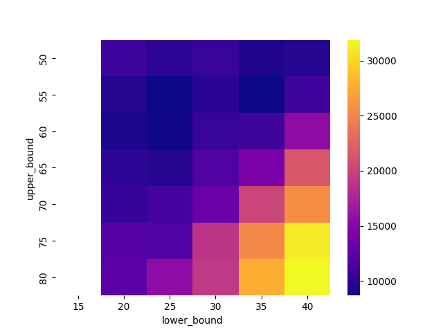
As a way of visualizing which parameter combinations perform best it can be nice to draw a heatmap comparing two variables and how changing them changes the metric you're optimizing for. You'll want to replace the code below your strategy definition with:
 1import matplotlib.pyplot as plt
 2import seaborn as sns
 3...
 4class RsiOscillator(Strategy):
 5    ...
 6...
 7
 8bt = Backtest(GOOG, RsiOscillator, cash=10_000, commission=.002)
 9
10stats, heatmap = bt.optimize(
11        upper_bound = range(50,85,5),
12        lower_bound = range(15,45,5),
13        rsi_window = range(10,30,2),
14        maximize='Equity Final [$]',
15        return_heatmap=True)
16
17# choose your colormaps from here
18# https://matplotlib.org/stable/tutorials/colors/colormaps.html
19hm = heatmap.groupby(["upper_bound","lower_bound"]).mean().unstack()
20sns.heatmap(hm, cmap="plasma")
21plt.show()
Since a heatmap can only display variations of two variables, we need to use a pandas group_by to select the two variables we want to compare against eachother. Then apply an aggregation to simplify each group down to a single value. Finally we unstack the whole thing into a matrix that we can easily plot with seaborn.
There's a whole host of color pallets available at the link in the code block above.

Multi-timeframe Strategies
For those of you fond of TA, we often want to examine a strategy on multiple timeframes. Say on the weekly and the daily. Thankfully there's a nice utility function called resample_apply. It leverages Pandas to down-sample the data, apply our indicator, then up-sample it and forward fill the missing values. Here's a re-written version of our init function that gives us the weekly rsi:
1# All initial calculations
2    def init(self):
3        self.daily_rsi = self.I(ta.rsiI, pd.Series(self.data.Close), self.rsi_window)
4
5        # This magical function does all the resampling
6        self.weekly_rsi = resample_apply(
7            'W-FRI', ta.rsi, pd.Series(self.data.Close), self.rsi_window)
All you have to do is feed in a pandas compatible timeframe, the function you want to apply, the data and any extra keywords that need to be passed into the function. At this point we can re-write our next function to make use of our weekly_rsi.
1def next(self):
2
3        if (crossover(self.daily_rsi, self.upper_bound) and
4                self.weekly_rsi[-1] > self.upper_bound):
5            self.position.close()
6
7        elif (crossover(self.lower_bound, self.daily_rsi) and
8                self.lower_bound > self.weekly_rsi[-1]):
9            self.buy()
Now we only trade if there's a crossover on the daily candles, and the weekly rsi is also above our threshold.
Take Profit and Stop Loss
You can add a stop loss or take profit level in both your long and short trades as follows
1def next(self):
2
3        price = self.data.Close[-1]
4
5        if crossover(self.rsi, self.upper_bound):
6            self.position.close()
7
8        elif crossover(self.lower_bound, self.rsi):
9            self.buy(tp=1.15*price, sl=0.95*price)
Here we set a take profit at 15% and a stop loss at 5%. Note that due to how backtesting.py works, the final profit from your trade might be slightly higher/lower than the level you'd expect. This is because it only executes trades on the next bar, so if the price moves significantly overnight, that will affect your backtest. If you need very granular stop-losses and take-profits I'd recommend using more granular intra-day data.
Extracting Trade Data
You can extract the series of trades made by the backtester for further analysis.
1print(stats['_trades'].to_string())
 1    Size EntryBar ExitBar   EntryPrice   ExitPrice    PnL      ReturnPct  EntryTime   ExitTime Duration
 20    27       373      422   362.67390     439.40  2071.60470   0.211557 2006-02-10 2006-04-24  73 days
 31    33       493      525   365.70996     415.46  1641.75132   0.136037 2006-08-03 2006-09-19  47 days
 42    24       862      925   561.83142     557.94   -93.39408  -0.006926 2008-01-23 2008-04-23  91 days
 53    29       987     1126   467.65344     371.28 -2794.82976  -0.206079 2008-07-22 2009-02-09 202 days
 64    19      1367     1424   547.68318     563.00   291.01958   0.027967 2010-01-25 2010-04-16  81 days
 75    22      1437     1534   501.98196     512.86   239.31688   0.021670 2010-05-05 2010-09-22 140 days
 86    19      1653     1740   573.94560     592.49   352.34360   0.032310 2011-03-14 2011-07-18 126 days
 97    20      1873     1913   573.12396     646.60  1469.52080   0.128203 2012-01-26 2012-03-23  57 days
108    20      2072     2129   655.95930     767.69  2234.61400   0.170332 2012-11-09 2013-02-04  87 days
Video tutorial
If you'd prefer a video tutorial, you can check out this video on my channel: